Here we will present some classical computer vision techniques on how to identify nearby vehicles and lane lines.

Video of result

Important files can be found here

• model.py (builds SVM classifier and trains on training data)
• Processor.py (overlaying processor that runs the pipeline on a video stream input)
• settings.py (settings for tuned parameters)
• Car_Detector.py (contains Car_Detector class that applies the model to detect cars and draws rectangular boxes on images)
• helpers.py (contains helper functions for feature extraction and sliding window implementation)

  Training data:

• Our training dataset consists of 17760 images. 8792 non-vehicles and 8968 vehicles. We split our training and validation sets with 80% 20% respectively. So our training dataset was ~14208 images. The data looks like this

Process:

1) Training data (model.py)

• Grab the training data and extract image paths and store them in the model class
• Train a linear Support Vector Machine (lines 54 - 57)
• Split the training data using train_test_split. Keep in mind that we are using training data as validation data, so there is some overfitting there. On a time series analysis it would be more robust to check a time-range and split validation data so that it has distinct times from the training data
• Normalize the training data using mean - std normalization, using scikit’s StandardScaler (line 49)
• Set the LinearSVC’s C parameter to 0.01 so that it’s predictions will be less attached to the dataset and able to generalize better
• Train the model on the data
• Save the LinearSVC (Linear Support Vector Machine) to a pickle file as well as other parameters and move to step 2 (line 79)

2) Car detection (helpers.py)

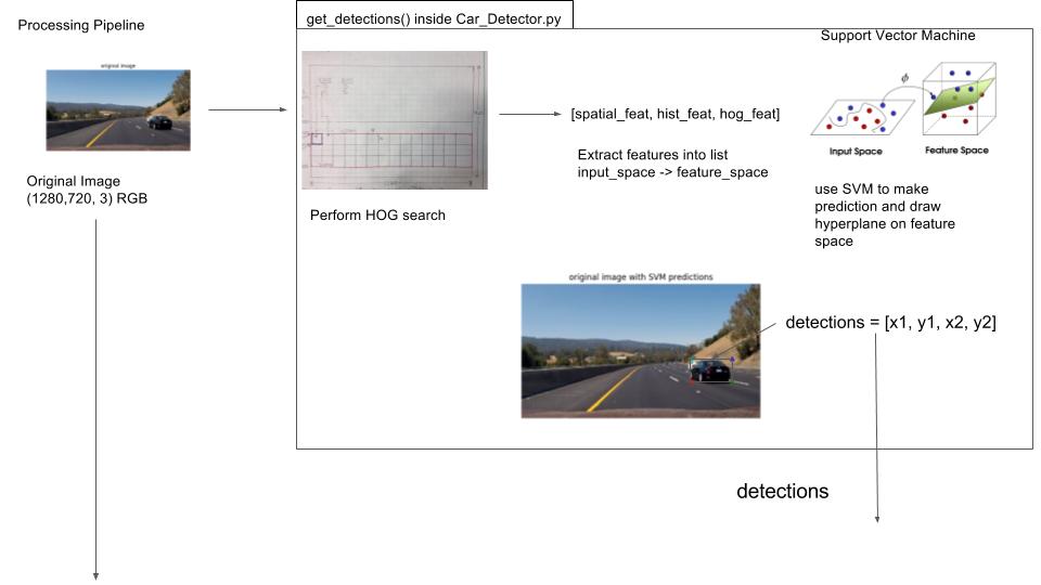
In Car_helpers.find_cars (helpers.py) implemented in get_detections() inside Car_Detector.py

Sliding Window Implementation

Instead of creating random sliding windows, extract features from an entire region of the image, and then use those cells to determine if there is a vehicle present.

• Extract out a section of the image (height from ystart to ystop as defined by the function caller in Car_Detector.py) and all width.
• Extract the HOG features for the entire section of the image
• Here is what HOG features gives us

• 
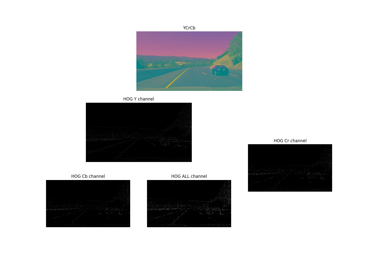
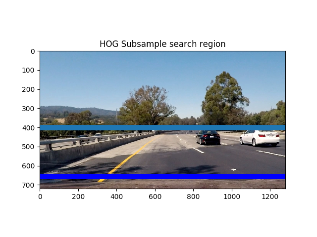
• Above: You can see the region we are using for our sub image between the light and dark blue lines
• Scale the extracted section by a scale parameter (line 168)
• Extract each channel from the scaled image
• Calculate the number of blocks in x and y
• Create multiple search windows with different scales and different regions (I used 3)
• Create a step size (cells_per_window / step_size) = % overlap
• Discover how many vertical and horizontal steps you will have
• Calculate HOG features for each channel lines
• Consider the scaled image to be in position space, not image space. We treat sections of the image as a grid in terms of whole integer values instead of in pixel values. See image below on how to grid looks

• We will move from grid space back into image space later on don’t worry
• For now, consider xpos and ypos to be grid positions (from left to right)
• Iterate through the grid (in y then x) lines
• Grab a subsample of the hog features corresponding to the current cell
• stack the features (line 203)
• go from grid space to pixel space now xleft and ytop are in image space
• extract the image patch (as defined by the boundaries of xleft and ytop and the window size)
• get the spatial and histogram features using spatial_features and hist_features which are defined in helpers.py
• Normalize the features using X_scaler from model.py
• Stack the features
• Compute the prediction from the Support Vector Machine and the confidence
• If the prediction is 1 and the decision function confidence is > 0.6 then we have detected a car
• Rescale xbox_left and ytop_draw to go from our current image space (which is scaled) to real image space by multiplying it by the scaling factor scale
• Use the drawing window dimensions to build (x1, y1, x2, y2) detection coordinates which will help us build a heatmap for the detected cars location
• Add those detections to our detections list

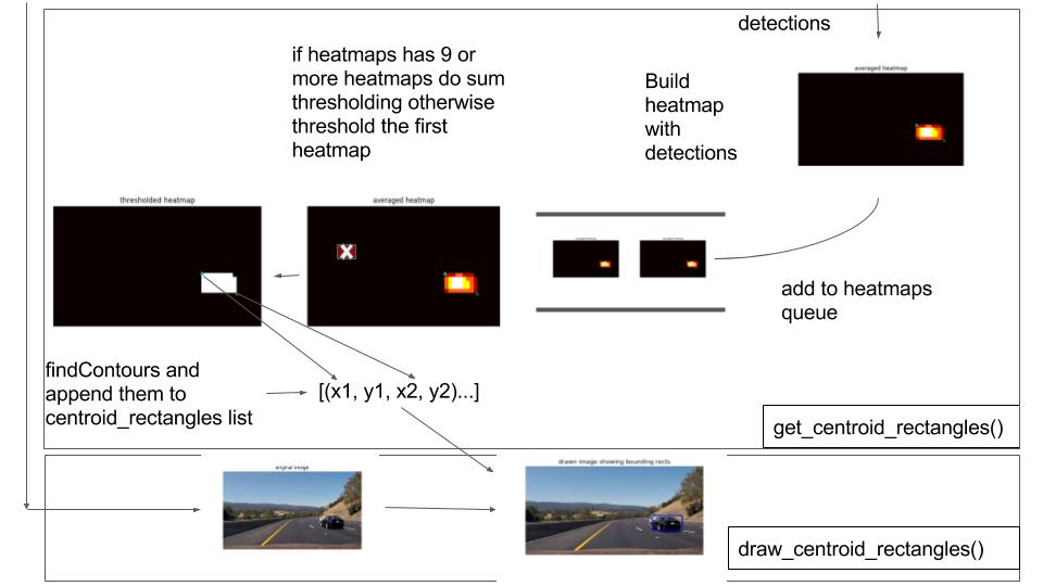
In Car_Finder.get_centroid_rectangles

• Take in the output from Car_Finder.find_cars (which are the detection coordinates above)
• Take in the detection coordinates and update the heatmap by adding 5 to each value within the heatmap’s bounding box
• 

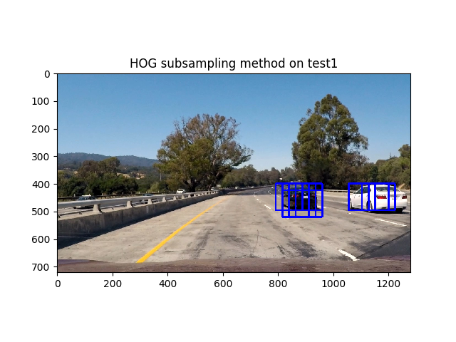
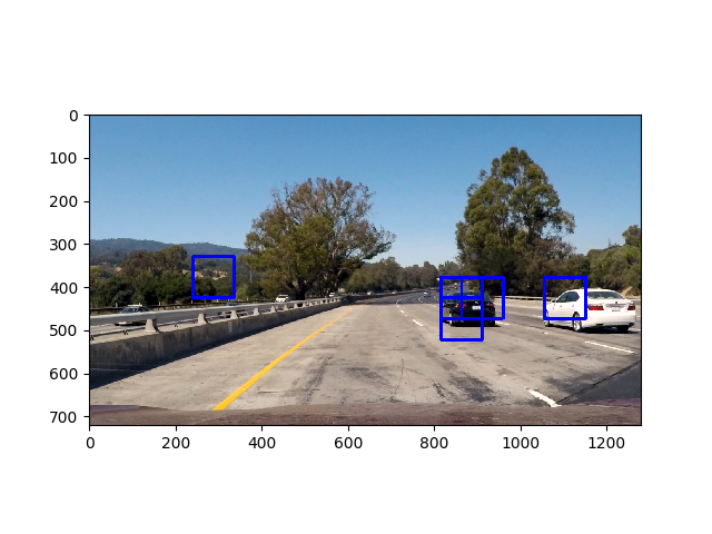
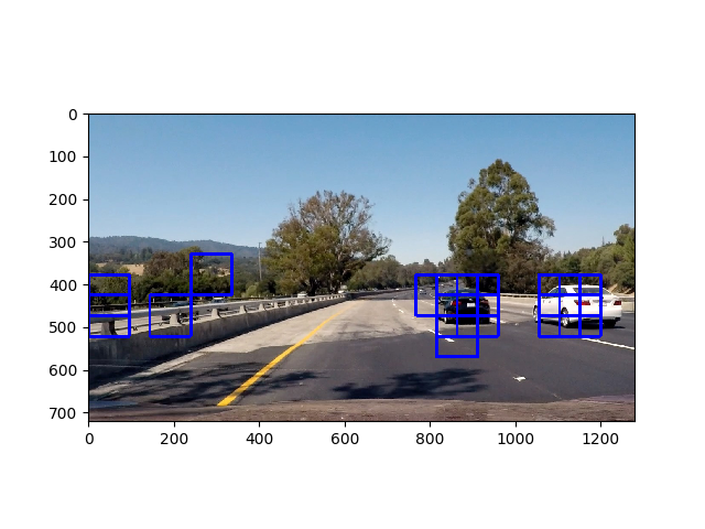
• Above, as you can see we have more than one bounding box. Therefore we need to apply a heatmap in order to determine an accurate region for the vehicle and only draw one box

• 
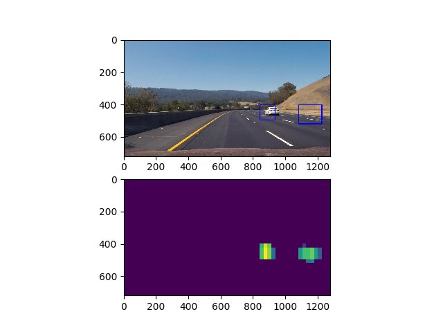
• As you can see, sometimes we get detections that are false positives, in order to remove these false positives we apply a thresholding function
• Remove the values where the heatmap’s values are < threshold. So it takes ~4 heat maps to pass through the thresholder
• Before we threshold, we take an average of the last 10 heat maps if 10 heat maps have been saved, then we insert this map into our thresholder
• Averaging allows us to rule out bad values and creates a smoother transition between frames
• Then we find the contours for the binary image, (which are basically the large shapes created from the heatmap)
• Then we create bounding boxes from these contours
• 
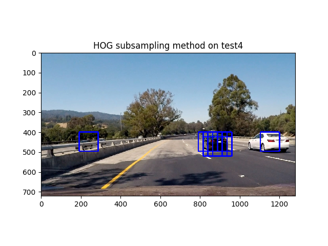
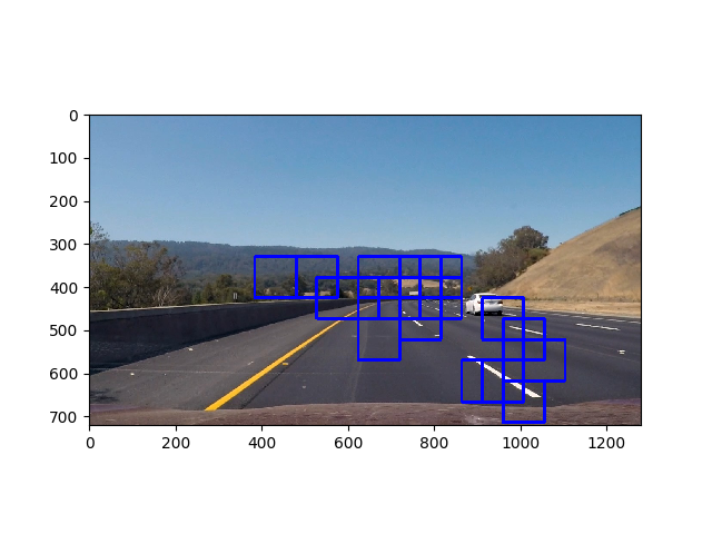
• Above you can see that we have some false positives in the opposing lane, therefore we will rule out any boxes that occur at width < 50 because this area corresponds to the opposing highway. We do this on line 91
• Grab the coordinates of the bounding box and append them to centroid_rectangles which we will pass to our draw_centroids helper function

  Draw Centroids (in helpers.py)

• Get the centroid coordinates and the original image and draw a rectangle with the coordinates given
• Return this image.
• Note: I got the idea to find the contours from Kyle Stewart-Frantz

Helper functions (in helpers.py)

• Extract_features (lines 61 - 112). This function takes in list of image paths, reads the images, then extracts the spatial, histogram, and hog features of those images and saves them. This occurs in our preprocessing pipeline when we are training the model. Our SVM does not extract features itself, so we have to extract them from images, similar to how a multi-layer perceptron works, in contrast with how CNN’s work.
• We extract features using three helper functions:
• bin_spatial : This function resizes our image to a desired size and then flattens it, giving us the pixel values in a flattened row vector
• color_hist: This function computes the histogram for each color channel and then concatenates them together
• get_hog_features: This function computes the histogram of oriented gradient and returns a 1-D array of the HOG features
• Then inside Extract_features we grab all of these features for each image and then add them to our features list. So features contains the features for the entire data set where a file_feature contains the features for one image THE END

Details (Parameter selection) (tuning params.ods)

Color Space:

• 
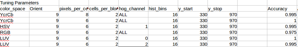
• Above: I tried these different parameters and tested the SVM’s predictions on a single image. I chose the YCrCb ALL channel color space because it gave me the best accuracy at training time
• 
• Above: Result of training using YCrCb color space
• This gives us the best result with an accuracy of 99.5. Don’t be fooled by the 1.0 in the grid of parameter tests, that was only sampled for one image
• 
• Above: Result of training using L channel in LUV color space
• 
• Above: Result of training using V channel in LUV color space

  Orientations:

• I chose to use 9 orientations

Performance Optimizations:

• I stored all my image paths in a pandas dataframe. I processed each image and viewed the results to see how well my pipeline works. When using the summing method, I started out with a threshold of 0.6 * 10 ~ 60. I later tuned this threshold to be 0.58 * 10 = 58. If I used 56 I would start drawing boxes in the middle of the road.
• I did not create a new image to draw on each time, I simply drew on the input image. I didn’t want to process more things.

Video of result

Video of lane line detection + object detection

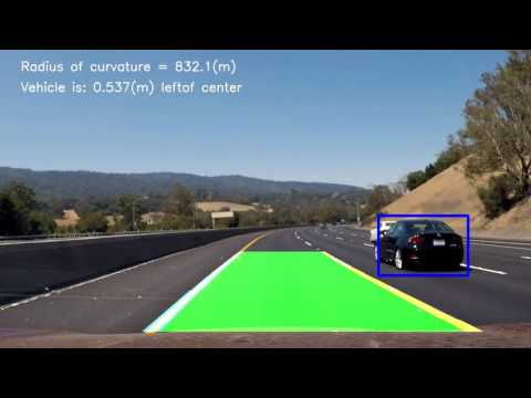
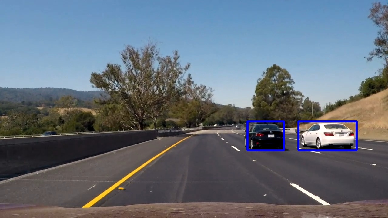
Final Result Image:

Reflection:

I tried a lot of different methods to get the most accurate pipeline. In theory, saving the state of the heatmap for subsequent images should work if you cool the regions where there are not current detections. This approach seems to work fairly well as you can see in the Video for heatmap cooling above. However, it involves storing more information because you have to save the state of the current heatmap to memory and it increases computation time. I like the idea of it, although determining the thresholds for it was rather difficult and involved a fair amount of evaluation.

The heatmap summming approach allows me to work with whole number thresholds instead of decimal thresholds (which are used in the averaging approach). Other than that it performs relatively the same as the averaging approach. I scaled the threshold value based on the number of heatmaps that are stored in the heatmaps queue.

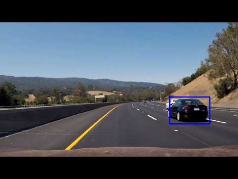
As I pass through the lightly colored road I lose a detection on the white vehicle. This is simply due to the model parameters and the prediction constraints. At this point I do not have an accurate prediction, so no bounding box is drawn. The model is only as good as the data.

At one point in the video the bounding box splits into two bounding boxes when it should be one bounding box. This happened because cv2.findContours found two contours due to the upper and lower section of the bounding boxes.

• 
• 
• (Above) as you can see in this case the cv2.findContours function inside get_centroid_rectangles detects two different contours, and that’s why two bounding boxes were drawn.

Twitter: @jonathancmitch

Linkedin: https://www.linkedin.com/in/jonathancmitchell

Github: github.com/jonathancmitchell

Medium: https://medium.com/@jmitchell1991

Tools used

• Numpy
• OpenCV3
• Python
• Pandas
• Matplotlib
• SciKit-Learn